Technology – ☆ Neuronenstern

Gaussian Procress Regression (GPR) is a powerful tool to do uncertainty estimation for all kinds of problems including state estimation in robotics or machine learning of geospatial data. It enables you to get an uncertainty estimation given new incoming data and is related to the concept of Kalman filtering that was briefly mentioned on this blog before. In this post I show the basic building blocks of this method and how to code a GPR yourself using Python.

Background

Formally, a Gaussian process is a stochastic process and can be understood as a distribution over functions. The premise of this approach is that the function values themselves are random variables. When modeling a function as a Gaussian process, one makes an assumption that any finite number of sampled points form a multivariate normal distribution.

Thus, $f(x) \sim GP(\mu, k)$ means that for any finite batch of function values $\mathbf{f} = f(\mathbf{X})$ , where $\mathbf{f} = \left[ f(\mathbf{x_1}, ..., f(\mathbf{x_n}))\right] \sim \mathcal{N}(\mu, K)$ holds.

One might ask why this assumption is useful. The main benefit of using Gaussian distributions is that they are incredibly nice to work with. The Gaussian family is self-conjugate and has a number of nice properties such as being closed under marginalization and closed under conditioning. This makes it a natural choice for Bayesian machine learning, where you have to specify a prior belief and then marginalize over parameters to obtain a posterior predictive distribution.

Also, the multivariate normal distribution is entirely characterized by a mean vector and a covariance matrix.

Inference

So how does one make predictions based on observed (training) data? It is basically based on this formulation:

(1) $\begin{equation*} \left[ {\begin{array}{c} f \\f^* \end{array} } \right] = \mathcal{N}\left( \mu, \left[ {\begin{array}{cc} K + \sigma^2 \mathbb{I}_n & K_* \\K_*^T & K_{**} \\ \end{array} } \right] \right). \end{equation*}$

The equation above reflects the previously mentioned assumption of normality, but here we also differentiate training and testing points (the latter is marked with an asterisk). There’s also an additional assumption that training labels are corrupted by Gaussian noise, which is the $\sigma$ part at the top left in the kernel-matrix above.

Now, it is possible to compute the conditional distribution of the test data:

(2) $\begin{eqnarray*} Cov(f^*) = K_{**} - K_*^T(K+\sigma^2 \mathbb{I}_n)^{-1}K_* \\ \mu(f^*) = K_*^T(K+\sigma^2 \mathbb{I}_n)^{-1}f. \end{eqnarray*}$

These equations give us a formal way of calculating the predictive mean and covariances at the test points conditioned on the training data.

GP Kernels

To actually use the equations above, one has to find a way to model the covariances and cross-covariances between all combinations of training and testing data. To do this we assume a certain kernel function for modeling the covariances. There are multiple possible kernels and choosing the right kernel function is critical for achieving good model fit, because they determine the shape of the resulting function. In this post I choose a squared exponential kernel: $k_{SqE}(x_1,x_2):= \sigma^2 \cdot \exp(-\|x_1-x_2\|^2_2)/(2 \cdot l^2))$ with $l>0$ the lengthscale and $\sigma^2>0$ the signal variance. But feel free to try out another kernels, like Brownian $k_B(x_1,x_2) := min(x_1,x_2)$ for example.

Once the hyperparameters are optimized, the kernel matrix can be plugged into the predictive equations for the mean and covariance of the test data to obtain concrete results.

Regression

One of the key features of GP regression is that we are modeling a function where we only have a limited number of observations. Yet, we are interested in the values (and uncertainties) at unobserved locations. This can be useful for weather prediction, as rainfall and temperatures are only measured at specific locations or for sensor readings that only occur every so often. Once you found a suitable kernel function for modeling the similarities between such data points distributed in space or time and you optimized the kernel function parameters using a training set, you can make predictions on the test set using the predictive equations.

Do it yourself with Python

Recall that I chose a squared exponential kernel, which itself is defined by a mean value $M$ and a variance $\sigma$ . We can quickly visualize this kernel to see what these two parameters do to the kernel.

Here is the kernel for our Python implementation:

class SquaredExponentialKernel:
    def __init__(self, sigma_f=1, length=1):
        self.sigma_f = sigma_f
        self.length = length

    def __call__(self, argument_1, argument_2):
        return float(self.sigma_f * np.exp(-(np.linalg.norm(argument_1 - argument_2)**2) / (2 * self.length**2)))

Let us shortly recall the formula:
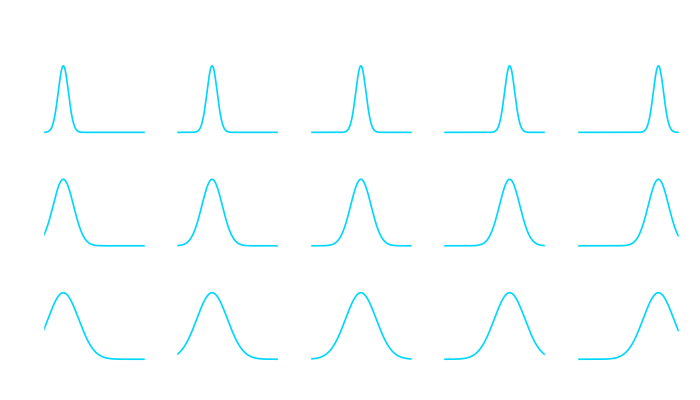
Given training points $x_1,...,x_n\in \mathbb{R}^m$ with values $y_1,...,y_n\in \mathbb{R}$ , $y = (y_i)\in \mathbb{R}^n$ with noise in each point $\mathcal{N}_{0,\sigma}$ and points $x_{n+1},...,x_k\in \mathbb{R}^m$ for which we want to predict the output, adapting our probability distribution leads to:

$\mathcal{N}(K_*^T(K+\sigma^2 \mathbb{I}_n)^{-1}f, K_{**}-K_*^T(K+\sigma^2 \mathbb{I}_n)^{-1}K_*)$ , with

$K= (k(x_i,x_j))_{i,j\leq n}$

$K_*= (k(x_i,x_j))_{n+1\leq i, j\leq n}$

$K_{**}= (k(x_i,x_j))_{n+1\leq i,j}$

And here we go with our main GPR class and a little visualization function:

# Helper function to calculate the respective covariance matrices
def cov_matrix(x1, x2, cov_function):
    return np.array([[cov_function(a, b) for a in x1] for b in x2])


class GPR:
    def __init__(self, data_x, data_y,
                 covariance_function=SquaredExponentialKernel(),
                 white_noise_sigma=0.0):
        self.noise = white_noise_sigma
        self.data_x = data_x
        self.data_y = data_y
        self.covariance_function = covariance_function

        # Store the inverse of covariance matrix of input (+ machine epsilon on diagonal) since it is needed for every prediction
        self._inverse_of_covariance_matrix_of_input = np.linalg.inv(
            cov_matrix(data_x, data_x, covariance_function) +
            (3e-7 + self.noise) * np.identity(len(self.data_x)))

        self._memory = None

    # function to predict output at new input values. Store the mean and covariance matrix in memory.

    def predict(self, at_values: np.array) -> np.array:
        k_lower_left = cov_matrix(self.data_x, at_values,
                                  self.covariance_function)
        k_lower_right = cov_matrix(at_values, at_values,
                                   self.covariance_function)

        # Mean.
        mean_at_values = np.dot(
            k_lower_left,
            np.dot(self.data_y,
                   self._inverse_of_covariance_matrix_of_input.T).T).flatten()

        # Covariance.
        cov_at_values = k_lower_right - \
            np.dot(k_lower_left, np.dot(
                self._inverse_of_covariance_matrix_of_input, k_lower_left.T))

        # Adding value larger than machine epsilon to ensure positive semi definite
        cov_at_values = cov_at_values + 3e-7 * np.ones(
            np.shape(cov_at_values)[0])

        var_at_values = np.diag(cov_at_values)

        self._memory = {
            'mean': mean_at_values,
            'covariance_matrix': cov_at_values,
            'variance': var_at_values
        }
        return mean_at_values


def plot_GPR(data_x, data_y, model, x, ax, color_index=1):

    mean = model.predict(x)
    std = np.sqrt(model._memory['variance'])

    for i in range(1, 4):
        ax.fill_between(x, y1=mean + i * std, y2=mean - i * std,
                        color=sns.color_palette('bright')[color_index], alpha=.3,)
        # label=f"mean plus/minus {i}*standard deviation")

    ax.plot(x, mean, label='mean', color=sns.color_palette(
        'bright')[color_index], linewidth=2)
    ax.scatter(data_x, data_y, label='data-points',
               color=sns.color_palette('bright')[color_index], s=30, zorder=100)
    
    pass

Now this is cool because now we can take a look at our GPR at work. The shaded areas represent 1,2,3 and 4 times the standard deviation. You can clearly see that uncertainty is low in the area where we have more data and it grows where we have no observations.

x_values = np.array([0, 0.3, 1, 3.1, 4.7])
y_values = np.array([1, 0, 1.4, 0, -0.9])
xlim = [-1, 7]
x = np.arange(xlim[0], xlim[1], 0.1)


fig, axes = plt.subplots(6, 1, figsize=(7, 9))
for i, ax in enumerate(axes.flatten()):
    x_val = x_values[:i]
    y_val = y_values[:i]
    model = GPR(x_val, y_val)
    plot_GPR(data_x=x_val, data_y=y_val, x=x,
             model=model, ax=ax, color_index=i)
    ax.set_xlim(xlim)
    ax.set_ylim([-6, 6])
plt.tight_layout()
plt.show()

Of course, we can also look at the different functions drawn from the distribution that make up our variance:

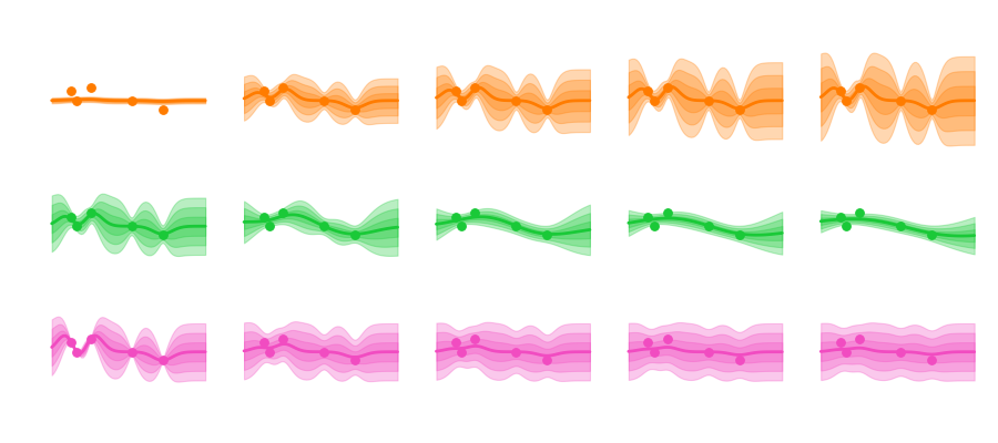
Another interesting aspect is that we of course still have the hyperparameters $\sigma$ , $l$ and the noise that can influence how we model our data. Varying these parameters looks like this:

Sigma mainly influences the uncertainty envelope, allowing for functions that more or less deviate from the mean. The length scale influences how smooth the curve becomes, and how curvy and bendy the functions get. And depending on the amount of noise we assume in the data the predicted functions are more or less tied to the observation points.

Conclusion

A GP model is a non-parametric model which is flexible and can fit many kinds of data, including geospatial and time series data. At the core of GP regression is the specification of a suitable kernel function, or measure of similarity between data points. The tractability of the Gaussian distribution means that one can find closed-form expressions for the posterior predictive distribution conditioned on training data. For a deep dive, feel free to look at the book Gaussian Processes for Machine Learning by Rasmussen and Williams.